Linear Regression

Linear modeling by the most elementary model : simple linear regression where a variable X is explained, modelled by an affine function of another variable y. Mostly used to predict continuous value outputs.

Introduction

First of all, what is linear ?

The term “linearity” in algebra refers to a linear relationship between two or more variables. If we draw this relationship in a two-dimensional space (between two variables), we get a straight line. In three dimensions it is a plane, and in more than three dimensions, a hyperplane.

In this example, we will use Scikit-Learn which is a Python machine learning library.

Goal

• Y the real random variable to be explained (endogenous, dependent or response variable)

• X the expanatory variable or fixed effect (exogenous).

• We assume that, on average, E(Y), is an affine function of X. Writing the model implicitly assumes a prior notion of causality in the sense that Y depends on X because the model is not symmetrical.

We want to predict a dependent variable value (y) based on a given independent variable (x). So, this regression technique finds out a linear relationship between x (input) and y(output). By ploting variables, linear regression gives us a straight line that best fits the data points.

So, what does the linear regression algorithm ?

It gives us the most optimal value for the intercept and the slope. Y and X can’t be changed since they are fixed data. The only values that we can control are b and m. The algorithm check for the line with the least error, that fits the most data points.

---

I - Simple linear regression

Basic linear equation :

\(Y = mx + b\)

• \(b\) : intercept

• \(m\) : slope

## Data from : https://www.kaggle.com/dronio/SolarEnergy?select=SolarPrediction.csv

import pandas as pd  
import numpy as np  
import matplotlib.pyplot as plt  
import seaborn as seabornInstance 
from sklearn.model_selection import train_test_split 
from sklearn.linear_model import LinearRegression
from sklearn import metrics

---------------------------------------------------------------------------
ModuleNotFoundError                       Traceback (most recent call last)
/tmp/ipykernel_1819/117542596.py in <module>
      3 import matplotlib.pyplot as plt
      4 import seaborn as seabornInstance
----> 5 from sklearn.model_selection import train_test_split
      6 from sklearn.linear_model import LinearRegression
      7 from sklearn import metrics

ModuleNotFoundError: No module named 'sklearn'

dataset = pd.read_csv('/Users/Laurine/Documents/Python Scripts/IMAC2/Learn-computer-graphics/Linear-Regression/SolarPrediction.csv')

## See data
dataset.describe()

	UNIXTime	Radiation	Temperature	Pressure	Humidity	WindDirection(Degrees)	Speed
count	3.268600e+04	32686.000000	32686.000000	32686.000000	32686.000000	32686.000000	32686.000000
mean	1.478047e+09	207.124697	51.103255	30.422879	75.016307	143.489821	6.243869
std	3.005037e+06	315.916387	6.201157	0.054673	25.990219	83.167500	3.490474
min	1.472724e+09	1.110000	34.000000	30.190000	8.000000	0.090000	0.000000
25%	1.475546e+09	1.230000	46.000000	30.400000	56.000000	82.227500	3.370000
50%	1.478026e+09	2.660000	50.000000	30.430000	85.000000	147.700000	5.620000
75%	1.480480e+09	354.235000	55.000000	30.460000	97.000000	179.310000	7.870000
max	1.483265e+09	1601.260000	71.000000	30.560000	103.000000	359.950000	40.500000

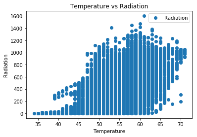
##  predict the maximum temperature taking input feature as the radiation.

dataset.plot(x='Temperature', y='Radiation', style='o')  
plt.title('Temperature vs Radiation')  
plt.xlabel('Temperature')  
plt.ylabel('Radiation')  
plt.show()

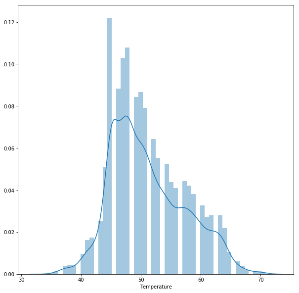
## We need to check the average temperature : we see that it is around 45 - 50

plt.figure(figsize=(10,10))
plt.tight_layout()
seabornInstance.distplot(dataset['Temperature'])

C:\Users\Laurine\Anaconda3\lib\site-packages\scipy\stats\stats.py:1713: FutureWarning: Using a non-tuple sequence for multidimensional indexing is deprecated; use `arr[tuple(seq)]` instead of `arr[seq]`. In the future this will be interpreted as an array index, `arr[np.array(seq)]`, which will result either in an error or a different result.
  return np.add.reduce(sorted[indexer] * weights, axis=axis) / sumval

<matplotlib.axes._subplots.AxesSubplot at 0x1d0ca426518>

## We need to divide the data into attributes (independant variables) and labels (dependant variables). Labels are values we want to predict
## Here, our attribute is "radiation" and our label is "temperature"

X = dataset['Radiation'].values.reshape(-1,1)
y = dataset['Temperature'].values.reshape(-1,1)

## We need to split the data between the training and the test set. Let say we give 70% of the data to the training set and 30 % to the test set

X_train, X_test, y_train, y_test = train_test_split(X, y, test_size=0.3, random_state=0)

## It is time to traing our algorithm ! 

regressor = LinearRegression()  
regressor.fit(X_train, y_train) #training the algorithm

LinearRegression(copy_X=True, fit_intercept=True, n_jobs=None,
         normalize=False)

## We found the best value for the intercept (b) and the slope (m)

#To retrieve the intercept:
print(regressor.intercept_)
#For retrieving the slope:
print(regressor.coef_)

[48.12878042]
[[0.01442639]]

## Time to make prediction ! (we need to use the test dataset and compare it to actual data)

y_pred = regressor.predict(X_test)
df = pd.DataFrame({'Actual': y_test.flatten(), 'Predicted': y_pred.flatten()})

df1 = df.head(30)
df1.plot(kind='bar',figsize=(20,20))
plt.grid(which='major', linestyle='-', linewidth='0.5', color='orange')
plt.grid(which='minor', linestyle=':', linewidth='0.5', color='orange')
plt.show()

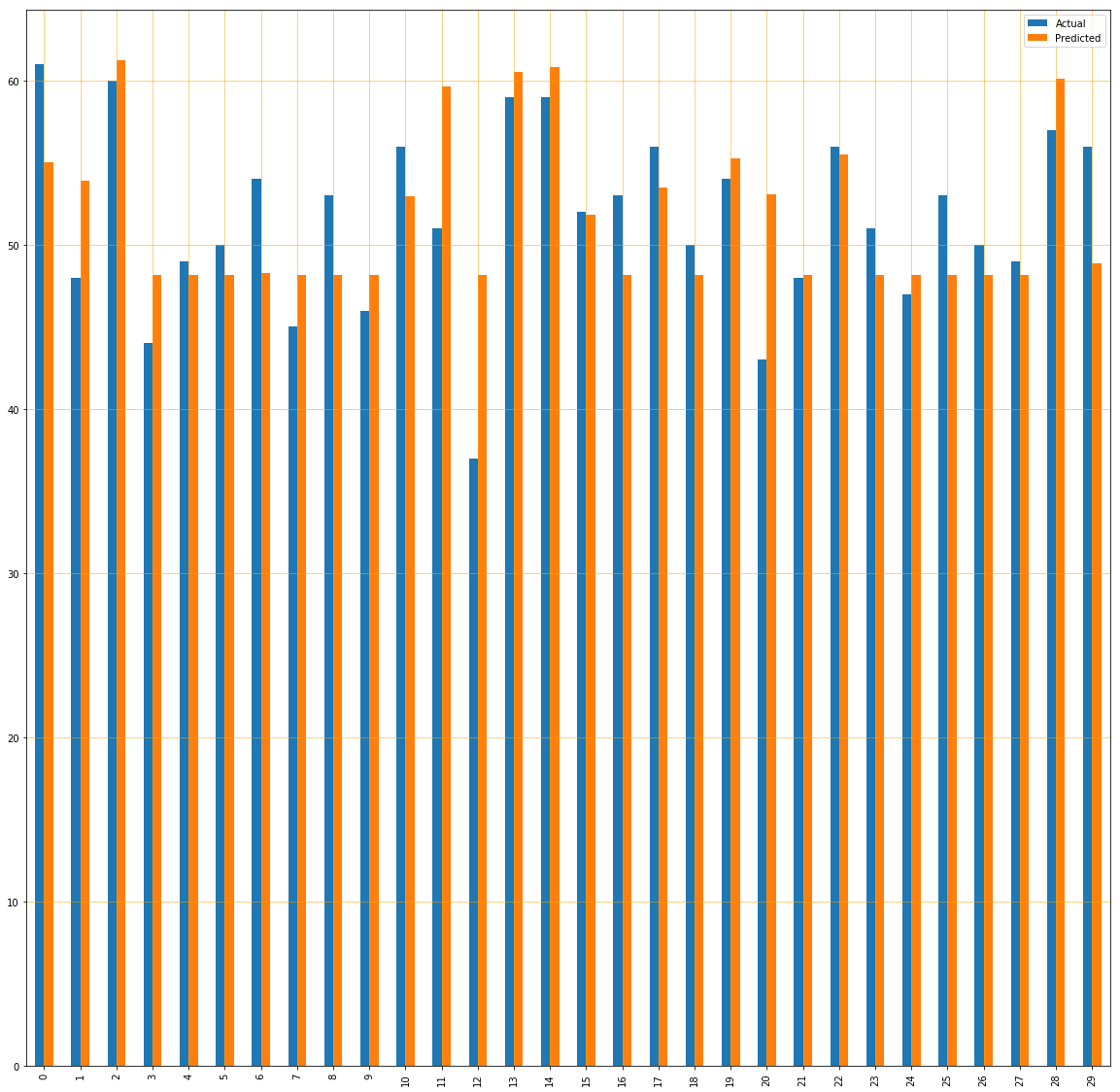
Predicted percentage are quite close to actual one, which means that our algorithm is well trained.

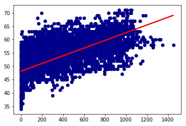
## Well, now it's time to plot our straight line ! 

plt.scatter(X_test, y_test,  color='darkblue')
plt.plot(X_test, y_pred, color='red', linewidth=2)
plt.show()

## The final step is to evaluate the performance of the algorithm. 

print('Mean Absolute Error:', metrics.mean_absolute_error(y_test, y_pred))  
print('Mean Squared Error:', metrics.mean_squared_error(y_test, y_pred))  
print('Root Mean Squared Error:', np.sqrt(metrics.mean_squared_error(y_test, y_pred)))

Mean Absolute Error: 3.3428145712086974
Mean Squared Error: 17.923509301005502
Root Mean Squared Error: 4.2336165746327925

You can see that the value of root mean squared error is 4.23, which is waaaaay above 10% of the mean value of the temperature (which is 45). This means that our algorithm is not accurate, but can still be used for a first approach.

So what if simple linear regression doesn’t work well ?

The best way to handle that is to choose the good amount of data and to train it well. Machine learning is all about that : training your model and realize that the training has not been good, that the predictions are not very accurate and start over again. Good luck !

---

II - Multiple linear regression

After performing a simple linear regression, you might wonder how to proceed with more than two variables. Steps for this linear regression is quite the same as above but the evaluation is different. It can be used to find out which factor has the highest impact of the predicted output and how different variables are related to each other.

The formula for multiple Linear Regression is : \(y_i = \beta_0 + \beta _1 x_{i1} + \beta _2 x_{i2} + ... + \beta _p x_{ip} + \epsilon\)

\begin{aligned} &\textbf{where, for } i = n \textbf{ observations:}\ &y_i=\text{dependent variable}\ &x_i=\text{expanatory variables}\ &\beta_0=\text{y-intercept (constant term)}\ &\beta_p=\text{slope coefficients for each explanatory variable}\ &\epsilon=\text{the model’s error term (also known as the residuals)}\ \end{aligned}

The multiple regression model is based on the following assumptions:

• There is a linear relationship between the dependent variables and the independent variables.

• The independent variables are not too highly correlated with each other.

• yi observations are selected independently and randomly from the population.

• Residuals should be normally distributed with a mean of 0 and variance σ.

Take a deep breath. We won’t directly use this formula, since we work with Scikit-Learn. However, it is always useful to understand what data you are manipulated, why and how.

# Now, let's start coding ! 
# Data from : https://www.kaggle.com/bappekim/air-pollution-in-seoul

dataset = pd.read_csv('/Users/Laurine/Documents/Python Scripts/IMAC2/Learn-computer-graphics/Linear-Regression/AirPollutionSeoul/Measurement_summary.csv')

# Let's see our data
dataset.describe()

	Station code	Latitude	Longitude	SO2	NO2	O3	CO	PM10	PM2.5
count	647511.000000	647511.000000	647511.000000	647511.000000	647511.000000	647511.000000	647511.000000	647511.000000	647511.000000
mean	113.000221	37.553484	126.989340	-0.001795	0.022519	0.017979	0.509197	43.708051	25.411995
std	7.211315	0.053273	0.078790	0.078832	0.115153	0.099308	0.405319	71.137342	43.924595
min	101.000000	37.452357	126.835151	-1.000000	-1.000000	-1.000000	-1.000000	-1.000000	-1.000000
25%	107.000000	37.517528	126.927102	0.003000	0.016000	0.008000	0.300000	22.000000	11.000000
50%	113.000000	37.544962	127.004850	0.004000	0.025000	0.021000	0.500000	35.000000	19.000000
75%	119.000000	37.584848	127.047470	0.005000	0.038000	0.034000	0.600000	53.000000	31.000000
max	125.000000	37.658774	127.136792	3.736000	38.445000	33.600000	71.700000	3586.000000	6256.000000

# Same as for the simple linear regression, we need to divide our data into attributes and labels. 
# X variable contains all the attributes/features and y variable contains labels.
# Let's say we want to predict the NO2

X = dataset[['Latitude','Longitude', 'SO2','O3', 'CO', 'PM10','PM2.5']].values
y = dataset['NO2'].values

# We need to check the average value of NO2

plt.figure(figsize=(10,10))
plt.xlim((0,1))
plt.tight_layout()
seabornInstance.distplot(dataset['NO2'])

C:\Users\Laurine\Anaconda3\lib\site-packages\scipy\stats\stats.py:1713: FutureWarning: Using a non-tuple sequence for multidimensional indexing is deprecated; use `arr[tuple(seq)]` instead of `arr[seq]`. In the future this will be interpreted as an array index, `arr[np.array(seq)]`, which will result either in an error or a different result.
  return np.add.reduce(sorted[indexer] * weights, axis=axis) / sumval

<matplotlib.axes._subplots.AxesSubplot at 0x1d0ab384f98>

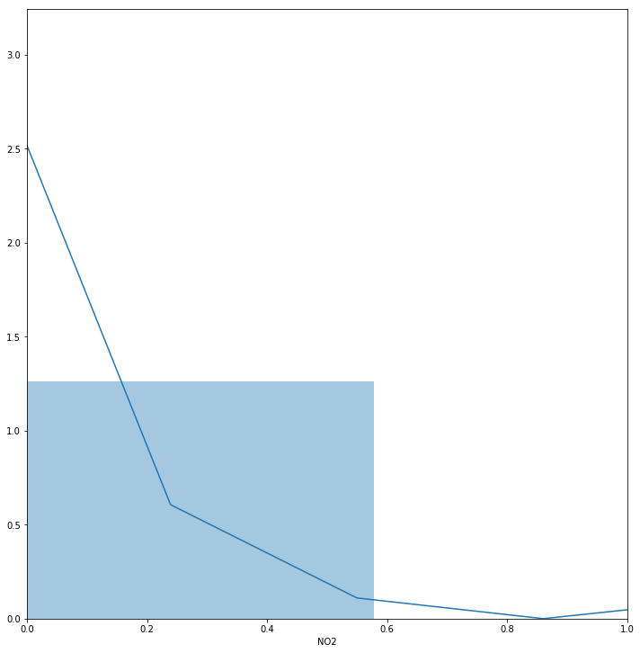
We see that the average of NO2 is something between 0.1 and 0.2

# Next, we split 70% of the data to the training set while 30% of the data to test set using below code.

X_train, X_test, y_train, y_test = train_test_split(X, y, test_size=0.3, random_state=0)

# Time to train our model ! 
regressor = LinearRegression()  
regressor.fit(X_train, y_train)

LinearRegression(copy_X=True, fit_intercept=True, n_jobs=None,
         normalize=False)

# We want to see what coefficient our regression algorithm has chosen
print('Latitude','Longitude', 'SO2','O3', 'CO', 'PM10','PM2.5')
print(regressor.coef_)

Latitude Longitude SO2 O3 CO PM10 PM2.5
[-5.63239684e-02  1.01338366e-02  2.52565384e-01  7.52547726e-01
  2.02347868e-02  1.35922634e-05  3.33477562e-05]

A unit increase in “Latitude“ results in a decrease of : \(-5.6 * 10^-2\) units in the NO2.

# Time to make our prediction : 
y_pred = regressor.predict(X_test)

# We need to check the difference between the actual value and the predicted one 
df = pd.DataFrame({'Actual': y_test, 'Predicted': y_pred})
df1 = df.head(25)

df1.plot(kind=’bar’,figsize=(10,10)) plt.grid(which=’major’, linestyle=’-’, linewidth=’0.5’, color=’green’) plt.grid(which=’minor’, linestyle=’:’, linewidth=’0.5’, color=’black’) plt.show()

Our model is quite bad at predicting but it could be worse. Remember : machine learning, once again, is all about training and testing your model.

## Well, now it's time to plot our lines ! 

plt.scatter(X_test[:,0], y_test, color='darkblue')
plt.plot(X_test[:,0], y_pred, color='red', linewidth=2)
plt.show()

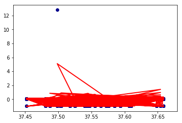
Well it is kinda chaotic since we have multiple variables but you can see that our lines cover our data well.

# It's time to evaluate our algorithm ! 
print('Mean Absolute Error:', metrics.mean_absolute_error(y_test, y_pred))  
print('Mean Squared Error:', metrics.mean_squared_error(y_test, y_pred))  
print('Root Mean Squared Error:', np.sqrt(metrics.mean_squared_error(y_test, y_pred)))

Mean Absolute Error: 0.01950224842895457
Mean Squared Error: 0.0013053866895743607
Root Mean Squared Error: 0.03613013547683375

Well actually the root mean squared error is 0.04. The mean value is something in between 0.1 and 0.2. It is a bit more than 10% of this range value but it is still very good ! We can make good predictions.

So what if multiple linear regression doesn’t work well ?

Maybe you need more data ? Maybe you thought that your data had a linear relation but it is not the case ? Maybe your training failed at some point ?

There is a lot of side-effect with machine learning. Remember : training and testing your algorithm is the best thing to do.

---

Conclusion

Congrats ! You’ve learn one of the most fundamental machine learning algorithms (thanks to Scikit-learn).